“How did we end up in today’s status quo, and where are we going?” This question constantly bothers me, but there must be a reason, right? Is it only me, or did software feel more responsive back in the day—“faster”—(and less buggy) than today, even though today’s hardware is hundreds of times faster? Surprisingly, even on my first PC, the early versions of Visual Studio are still starting up faster than the latest version on a really beefy machine.
Game developers are my favorite example—they are constantly pushing the limit of what’s possible within 16.7 milliseconds (or 11.1 ms for VR), squeezing so much computation, while at the same time, others are not even bothered when their web apps are not responding within, say, a second. That’s about 62 times longer!
There is a famous quote from Niklaus Wirth that states, “Software is getting slower more rapidly than hardware becomes faster.” Let’s pause here for a moment and let that sink in…

With this article, I would like to draw everybody’s attention to performance, explain how to monitor it, and provide a good introduction to something that I’m afraid is starting to seem like an enigma—profiling.
Why to profile?
How do you know if you have “performance issues”? Naturally, you can say it “feels slow” or “janky”, but that’s a really subjective statement. Moreover, how would you know whether today’s build is “better” than the last one you were running?
The act (or process) of measuring and collecting “(performance) metrics” is called profiling, hence the tool doing this job is called “profiler”. Collecting metrics alone won’t give you much insight since performance is relative.
As in any scientific process, we must do our due diligence to ensure they are collected reliably and in a deterministic fashion. We need to trust our measurements! First, we need to carefully choose the “metrics” to maintain a good enough signal-to-noise ratio—collecting everything is counterproductive. Second, we need to control the environment together with external “variables”.
Profilers are not magic. They will not tell you how to make your code run faster. They are only a tool that helps spot elephants in the room: bottlenecks and hotspots—the “longest running parts” of your code. Those will be your “suspects”, and you, as a detective, will have to start the investigation from there.
Different types of tools
Not all profilers are created equal, so choosing the correct tool for the job is a very important first step. There are basically two types of profilers, each with its own strengths and weaknesses.
Sampling profilers
Those are the simplest—they are just “spying” on our application and recording the footprints very often. Literally, they attach to our process and periodically, with a high yet fixed frequency, look at the stack trace (or at least the instruction register) of our application. This way, during the “recording” process, a sampling profiler collects many samples and runs some statistical analysis on them. What we end up with is a “trace” that shows how many times the program was “caught red-handed” executing a particular instruction.
The best thing is that sampling profilers work with any application without any modifications required. Those spies are so good that the app might not be aware that it’s being watched. All we have to do is run the profiler (collector) on the same device as our app.
The biggest drawback, in my opinion, is the averaging process and depth of the “collected intelligence” (we have less control over which metrics are collected), which makes it harder to spot the outliers or occasional hiccups. There’s also a particular drawback caused by the way those profilers work—they require the processor to run, so be careful when you put your cores to sleep.
Let me mention some of the best players in this category: Intel vTune, AMD μProf, Event Tracing for Windows, and Very Sleepy. It’s not surprising to see top-tier hardware manufacturers release their own tools. Many modern CPUs have internal hardware counters that allow us to collect really low-level metrics, such as the number of L1 or L2 cache misses! But in this category, you will also find the “Instruments” from Xcode (like Time Profiler) and the Android Profiler. GPUs are also not different here. A few notable mentions are NVIDIA Nsight, Radeon GPU Profiler, Intel GPA, and PIX!
Instrumentation-based profilers
This type of profilers requires your help and involvement. You need to modify your applications by “instrumenting it”—adding a small piece of code at the beginning (and sometimes at the end) of your functions and methods. It means you usually end up with a dedicated build tailored for profiling.
The best thing about instrumentation-based profilers is that you can have a lot of measurements available, not only “start” and “stop” times. As you modify your source code, you can wrap your locks (like mutexes and semaphores), allocators, etc., and then use all those data points to your advantage. Moreover, profilers that are tailored for games usually have a concept of a frame, which you can use in any way you want. Basically, you add a marker at the end of a “frame”, and now you can do frame-by-frame analysis and spot “frames” that are lagging or out of budget.
Here are some more advantages of this type of profilers:
- immune to compiler optimizations (like inlining)
- zones and markers can be labeled (and often colored to your liking)
- profiling can be turned on and off at any time, or stay always on
- do not require an external process for collecting
Examples of instrumentation-based profilers include RAD Telemetry, Tracy, Optick (previously known as Brofiler), and systrace.
Many profilers support both sampling and instrumentation-based ways of collecting metrics.
Preparing to profile
It might be very tempting to just go and run your app under a profiler, but… Do you really know what you want to achieve? What metrics are you collecting? Are you sure that your measurements are reproducible? How would you know whether something is “slow”? What does “slow” even mean?
If you have two measurements—let’s call them “baseline” and “current”—you can compare them and see that something is faster or slower, right? But how fast should it go? What’s fast enough? How would you know that you reached the ceiling? Do you have a budget defined?
I’m not trying to be picky here. Those are really important questions! We need to develop a plan and a reproducible process and set some hypotheses so we can test and verify each of them. It might sound familiar, but this is the core of the scientific process!
There are so many things that can hurt our app’s performance. Maybe we have a couple of singletons that operate on a shared state and had to be protected by a lock? Perhaps we are constantly allocating something on the heap and then throwing it away? We can be I/O bound, where the CPU idles while waiting for network requests to finish. It can go even worse, like when our app is memory bound, which is a sign of poor memory layout, lack of data locality, or random/unpredictable memory access patterns—those basically “turn off” all the optimizations built-in into our CPUs!
As you can see, we still need some domain knowledge. Not only do we need to know how our application is structured, but ideally, we should have at least some intuition on how the hardware works as well. The latter will help us tremendously to identify the root cause of any slowdown and turn such findings into actionable optimization steps. How would you otherwise figure out that your atomics are too close to each other and you suffer from false sharing? But let’s leave microarchitecture optimization topics for a different article.
Let’s check an example
This article might have gone a bit theoretical and dry. I know that in theory, there’s no difference between theory and practice, but in practice, there is… So, let’s get our hands dirty, shall we?
Let’s say I was tasked with creating a C++ Turbo Module for React Native that does simple image manipulations on a pixel-by-pixel basis. I promise not to open the Pandora box and drag you into the Digital Signal Processing wonderland. Let’s say I want to limit myself to simple linear transformations like adjusting brightness and contrast. Oh, and to spice things up, keep in mind that I’m suffering from the Not Invented Here syndrome, so no Frame Processors this time!
For profiling, I’ll use Tracy, an open-source and cross-platform profiler. It’s a single, self-sufficient 29MB file! I will walk you through the steps of setting it up, followed by instructions on how to instrument your source code and how to profile your code.
For simplicity’s sake, let’s imagine that no GPUs or shaders exist. We will stick to single-threaded code as well. In the end, if we make it faster on a single thread, it’s going to be even faster when run on multiple cores (but don’t take my word for granted; remember to measure and verify it yourself).
Getting the tool
You need to grab yourself a fresh clone of Tracy’s source code from GitHub. As there are no precompiled releases, you need to build the server app yourself. It uses CMake, so it’s just a matter of issuing two commands from your Terminal of choice:
For the client part, that would go into your app… Everything you need is inside the public directory. You can copy all the files to your project and only build TracyClient.cpp file—it will include everything you need.
Let’s go back to our app.
What slows down brightness and contrast adjustments?
Well, what can go wrong? Changing brightness is just adding (or subtracting) a constant from every pixel’s value. Adjusting contrast boils down to basically multiplying every pixel with another constant. As mentioned above, even though there are no data dependencies between iterations, we will stick to single-threaded execution.
Let’s take a quick look at the naive implementation.
Pretty straightforward, right? Each method does exactly one thing (separation of concerns), and we (almost) got rid of all code duplication (DRY)!
Note that I’ve added a ZoneScoped; line at the beginning of each function. This single line is the “instrumentation” that we have to add to make the function visible in the profiler! It records the start time during initialization and the stop time when the scope will be left.
Tracy also provides different variants of this macro. ZoneScopedN(“Your name”) can override the function’s inferred name to anything of your liking. Another one I found myself using a lot is ZoneScopedNC(name, color). Check out the official documentation for more.
You also need to include Tracy’s header file at the top of your cpp file:
Lastly, you need to add a preprocessor macro/define named TRACY_ENABLE (there is no D at the end!) to your project’s build settings. Without this macro, Tracy won’t be included in your build.
Let’s run our app! For simplicity’s sake, I’m running it in a simulator. It might not be the best choice, but it is still a good starting point.
Wait, where can I see the metrics?
Connecting the profiler
Tracy uses a client-server architecture. For practical reasons, your instrumented app (client) will only collect the metrics and send them over the network to your laptop (server) for analysis and storage. So, you start the UI on your laptop and connect to your instrumented app. All you need is the IP address of the profiled device! That’s well, though, isn’t it?
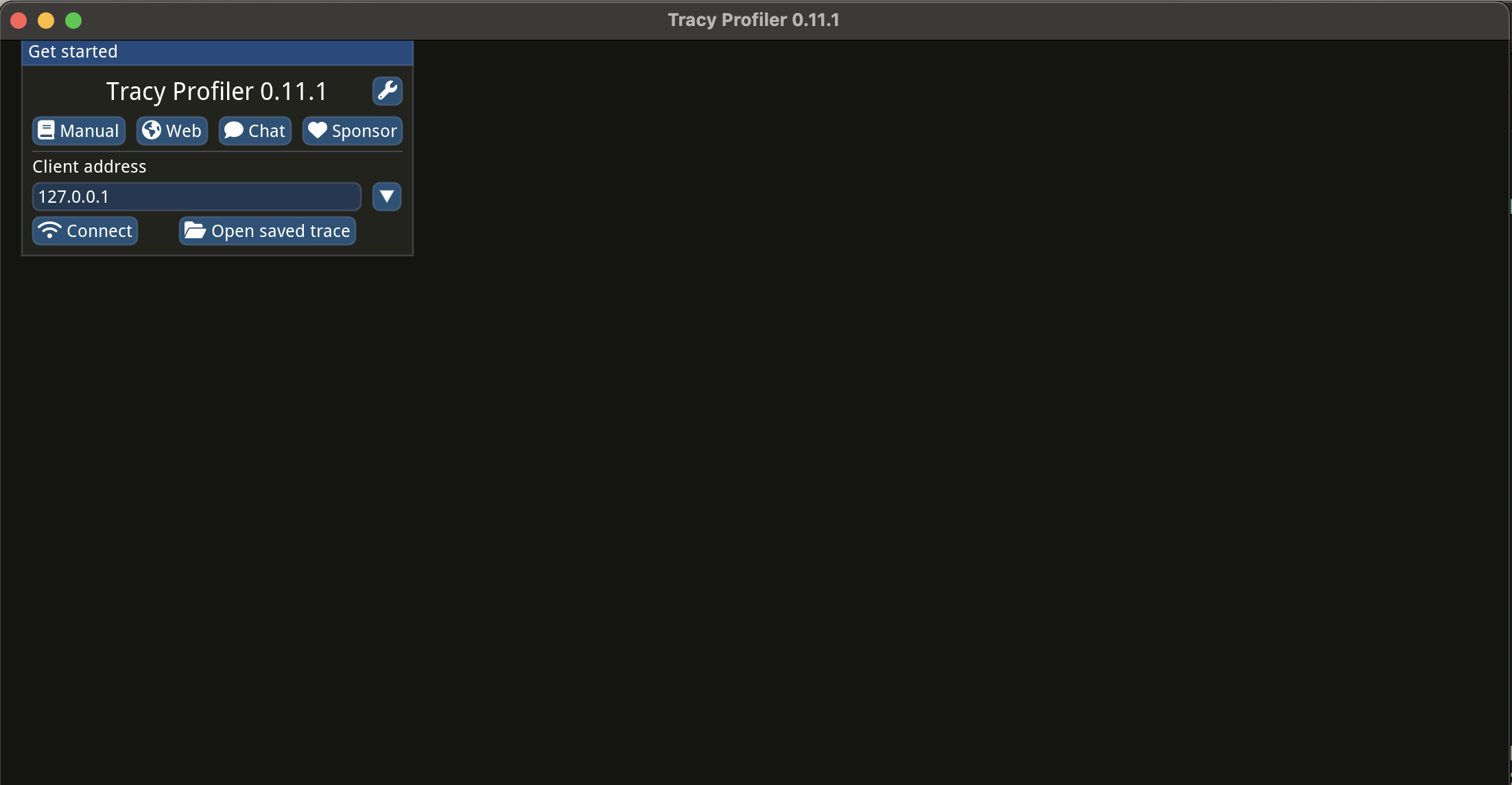
Leave the localhost IP address as it is and simply press the “Connect” button. Now that we see the data flowing and have some numbers, what should we do with them?
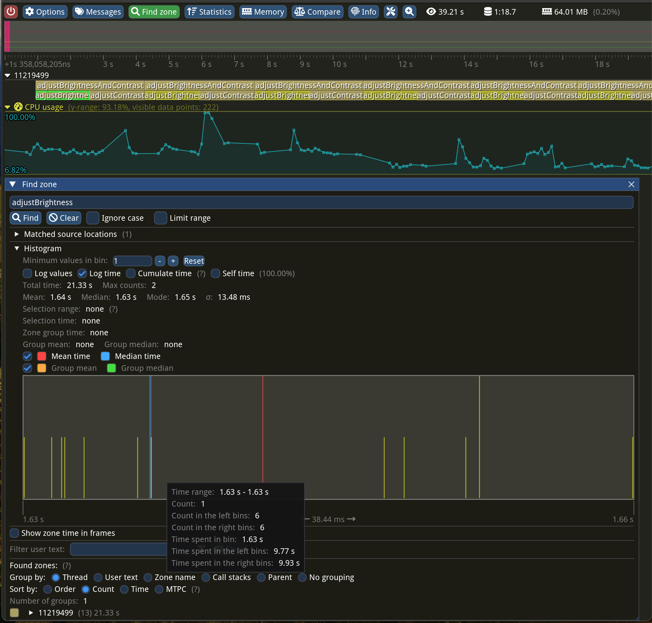
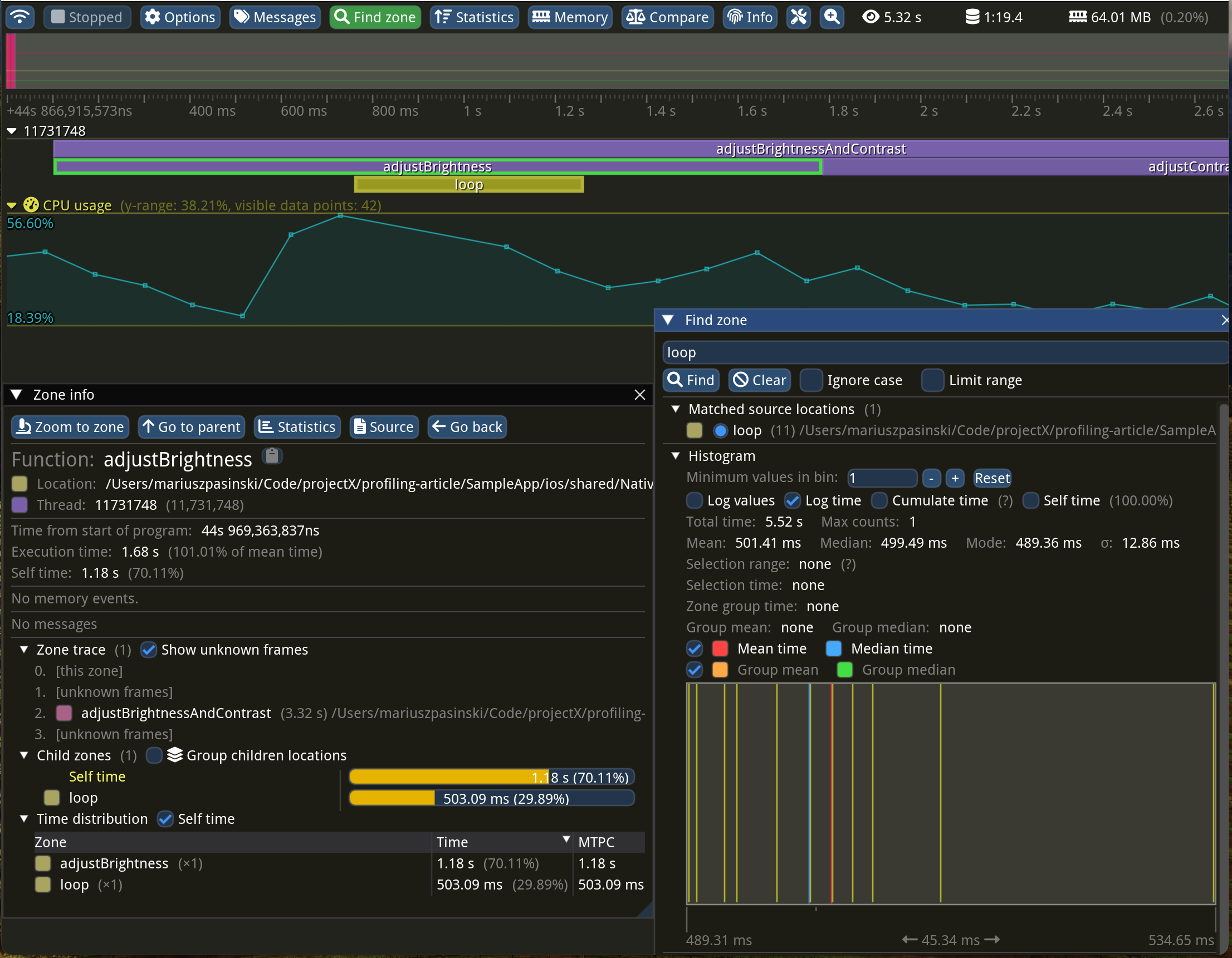
Let’s look at the adjustBrightness method, as it should be the fastest (only addition per pixel). The whole function was running a whooping 1.64 seconds on average! Adjusting both brightness and contrast takes 3.29 seconds…
The “Find zone” window at the bottom displays a nice statistical summary for a zone with a given name and a histogram plot! The more samples you have, the more it would resemble a bell curve. Just above this plot, you can see “Mean: 1.64 s” followed by “Median: 1.63 s”. The sigma letter denotes the standard deviation of 13.48 ms—the lower the number, the less noisy the measurements. You can search for zones by typing their names or pressing one in flame graph view and then clicking the “Statistics” button at the top of the “Zone info” window.
What’s the limit?
What if we have reached the hardware limits, and all we can do is ask the user to buy a newer, faster phone? How fast can we go, and how can we estimate this limit?
Just by looking at the code, we can notice that we are iterating over an array and doing simple operations. Let’s imagine we have a Full HD picture (that’s 1920 x 1080 pixels). Each pixel is stored on 4 bytes, one byte for each color channel: Red, Green, Blue, and Alpha, so our loop’s body is executed 8 294 400 times. Yup, this image takes 8100 KiB of memory! And yet, nowadays, we are taking even bigger pictures!
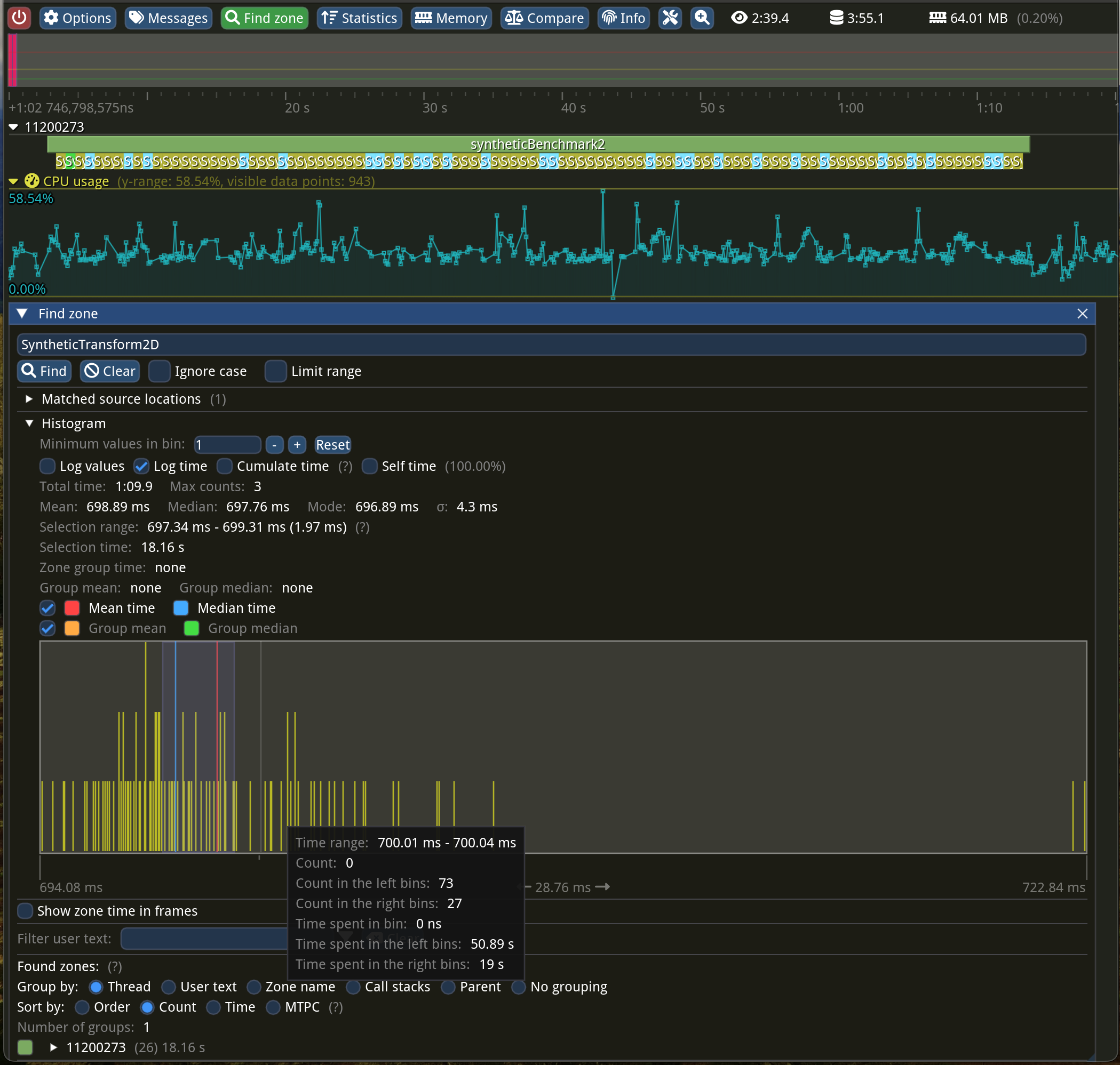
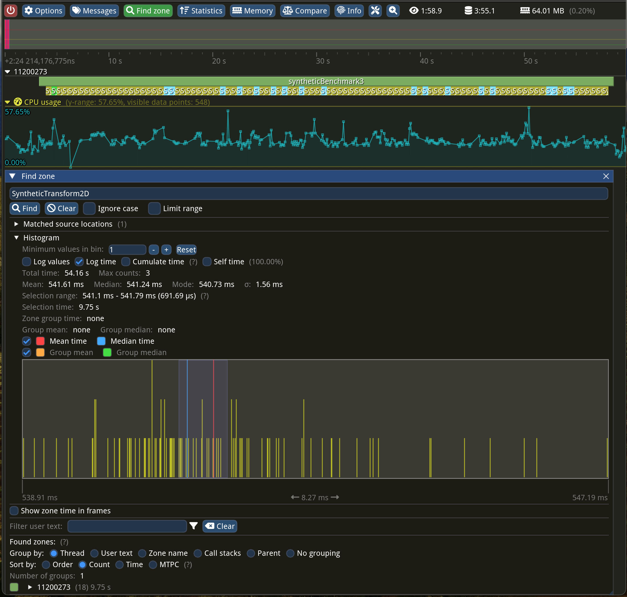
Let’s write a synthetic benchmark and keep it as simple as possible, allocating a big enough array and trying to apply a similar operation the same amount of times. We will repeat this test a couple of times just to get more reliable numbers. If our solution has similar numbers (same order of magnitude), then we cannot do much…
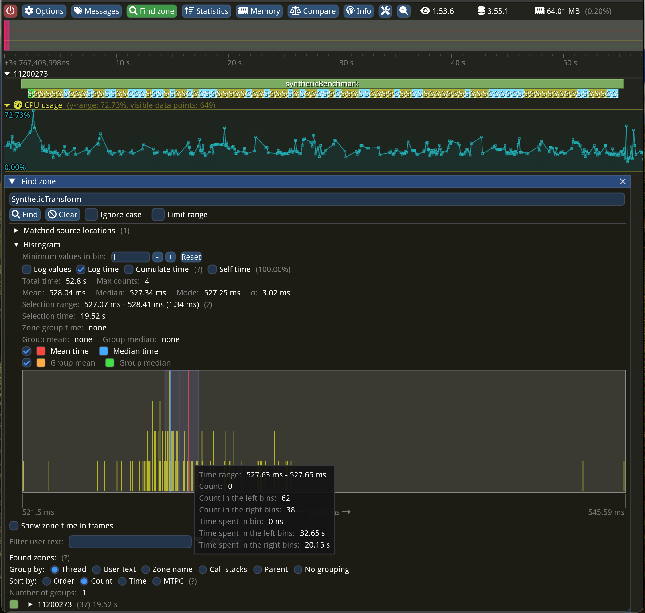

What just happened here? How come both multiplication AND addition run faster than just addition within our brightness function? For the same number of iterations, we went from 1.64 seconds to “just” 528 milliseconds—that’s 310% faster! Is it because three loops are more expensive than one?
For the uninitiated, pitch is the distance (in bytes) between subsequent rows. In our case, it’s just the width of the image times 4 bytes, but in some rare cases, there might be additional padding for alignment.
Why is this slower? Okay, I don’t want to prolong the article any further. It’s because of our suboptimal memory access pattern! CPUs are getting really fast at a much higher pace than memory. The performance gap between them is getting bigger and bigger!
So, what’s wrong with our memory access pattern? Well, CPUs do not access memory on a per-byte basis. They fetch the whole cache lines, which happens to be 64 bytes long in most cases. We are processing our image data column-wise instead of row-by-row. This makes the CPU read the whole cache line just to operate on 4 bytes, throwing away the remaining 60 bytes—what a waste!
To make as much of this cache line fetching, we want to process all those 64 bytes. 64B divided by 4B per pixel gives us 16 pixels. You might not believe it, but all we need to do is switch the order of the loops! Crazy, isn’t it?
You may also notice that in this version, we can skip recomputing the i constant in the inner loop. We can “hoist” it from both of these loops, turn it into a variable, and increment it in the inner-most loop.
Yes! We are back on the fast lane!
There are two additional things that I haven’t mentioned:
- This access pattern opens another optimization opportunity that has been implemented in hardware for at least a decade. CPUs can prefetch the “next” cache line for us before it’s needed if, and only if, we have a predictable pattern!
- Because our pixel data is tightly packed and we are iterating over adjacent pixels, our compilers should be able to benefit from that fact and auto-vectorize our code using SIMD instructions! In layman’s terms, the CPU can modify multiple data using a single CPU instruction!
Sweet, case closed! We identified the bottleneck in our first case! I’m leaving some low-hanging fruit as an exercise for the reader. I can give you a small hint, though: code duplication can be beneficial.
Now that we have learned something, we can go and optimize our original function!
In the next installment, I would like to share more tips and tricks regarding profiling (and optimizing) multithreaded applications! Surprisingly, lock contention is not as rare as I would like it to be…
PS: One more mystery for you: What else does our original function do besides running the loop? It looks like it spends 70% of its time doing something else… Any clues?


Learn more about Performance
Here's everything we published recently on this topic.